2 Jan 2026

Logistic Regression, the Sigmoid, and Log Loss

Mateo Lafalce - Blog

While standard linear regression is designed to predict a continuous numerical value, such as a person's height, logistic regression is designed to predict the probability that a given input belongs to one of two specific classes. These classes are typically coded as 0 and 1.

For instance, if the model accepts medical data as input and outputs 0.85, it is saying there is an 85% probability that this instance belongs to class 1.

To make a final classification decision, a threshold is applied to this probability. Typically, if the predicted probability is greater than 0.5, the model classifies the instance as 1; otherwise, it classifies it as 0.

Why Use the Sigmoid Hypothesis?

Logistic regression starts similarly to linear regression: it calculates a weighted sum of the inputs. The result of this calculation, often denoted as , can range anywhere from negative infinity to positive infinity ().

This presents a problem: probabilities must exist between 0 and 1.

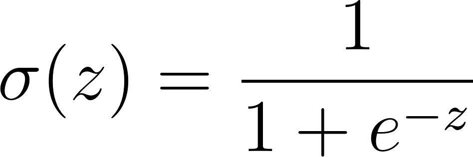
To solve this, we must transform that raw linear output  using a squashing function. We use the Sigmoid function. This function takes any real number as input and maps it to a value strictly between 0 and 1.

Sigmoid hypothesis

There are several crucial reasons why the sigmoid is the standard choice here:

• Bounding: It perfectly compresses outlier values. An incredibly high positive input yields a result very close to 1, while a very low negative input yields a result very close to 0.
• Differentiability: training in ML involves finding the best weights for the model using optimization algorithms like Gradient Descent. These algorithms require calculating derivatives. The sigmoid function is smooth and continuous, making these calculus operations efficient and stable.
• Clear Decision Boundary: The function is steepest around its center. This means the model is highly sensitive near the decision border, quickly pushing predictions toward certainty (0 or 1) as data points move away from that border.

Measuring Error: The Log Loss Function

Once the sigmoid function provides a predicted probability, how do we know if the model is doing a good job?

We need a Cost Function to measure the error -> the difference between the prediction and reality.

In linear regression, we typically use Mean Squared Error. However, if we use that method with the curved sigmoid function, the resulting error landscape becomes wavy, filled with many false valleys where the training algorithm can get stuck.

Instead, logistic regression uses Log Loss (or Binary Cross-Entropy). This method doesn't measure physical distance; it measures variance using logarithms.

The intuition behind Log Loss is to heavily penalize confident mistakes. If the model predicts a 99% chance of an event happening (), but it does not happen (), the error shouldn't just be moderate; it should be massive because the model was arrogantly wrong.

The logarithmic curve ensures that as a wrong prediction approaches certainty, the cost approaches infinity.

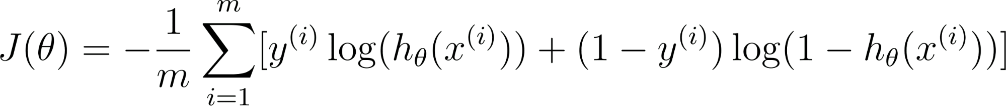
While the cost is calculated conditionally based on whether the true label is 0 or 1, these conditions are combined into a single, elegant mathematical equation for computational efficiency over an entire dataset of  examples:

This formula acts as a mathematical switch.

If the actual value  is 1, the second part of the equation cancels out. If  is 0, the first part cancels out.

This ensures that the model is always penalized correctly according to the true label. The goal of training is simply to find the model parameters that minimize this final  value.

This blog is open source. See an error? Go ahead and propose a change.